The SFT Code: Finalised!

I finally have good versions of the code, which have passed every test I know!

One version is very slow, but very accurate. It runs with a time step of 0.9 seconds only, which gives us a runtime of 325 days for a simulation of 11 years i.e. one sunspot cycle. This code can be used for observing small scale features which do not exist for long.

The faster version of the code runs with a time step of 250 seconds, which gives us a runtime of 24 hours per sunspot cycle. In this code, the grid points within 4.32 degrees of latitude from the pole have 50 points in the toroidal direction, whereas the rest of the latitudes have 1000 points in the toroidal direction.

The evolution of the radial field is second order accurate in both forms of the code, and there is a slight flux imbalance due to numerical round off, which is less than 0.1 % of the total flux.

I ran a simulation with the modeled sunspot input for one solar cycle, and the output is shown in the video here.

A Working Code with a New Grid

The Grid used for calculations in all previous codes was:

theta= 0 to pi in 501 steps, with a step-size of h=pi/500.
i.e. theta=linspace(0,pi,501)

This grid includes both the poles (theta=0 and pi) and the equator as grid points.

The corresponding area grid took into account the area surrounding these points. i.e. the area between theta-h/2 and theta+h/2.  So, the area corresponding to the point just after the pole would lie between the colatitudes of h/2 and 3h/2, and would look like a trapezium. Whereas, the area corresponding to the polar grid point would lie between colatitudes 0 and h/2, and would look like 2 triangles with a common vertex, and a common axis of symmetry. And the area-grid of the points on the equator lied equally in both the hemispheres.
The main problems we faced due to this grid, were that

1. there were terms in our master equation, that involved 1/sin(theta). These terms blew up at the poles.
2. The problem of flux transport over and across the poles (singularity).

Solution: Shift the grid by h/2.

The grid was shifted by h/2, such that it did not include the poles or the equator, or any integral multiple of pi/2. The new grid is:

theta= h/2 to pi-h/2  in 500 steps, with a step-size of h=pi/500.
i.e. theta=linspace(h/2,pi-h/2,500)

The corresponding area grid, includes triangular area for the points next to the pole, but now there is only one triangle on one side of the pole between colatitudes 0 and h, so we don't have to worry about flux crossing the poles. (Because the transport of flux in the area grid occurs between 2 areas with common side. But at the pole, the contact between 2 areas in the theta direction is through a single point, which gives us no flux transport across the pole. This is also theoretically verified.).

And the 1/sin(theta) terms in equations do not blow up because there is no grid point exactly at the poles.

So, our purpose of solving the issues is served with a shifted grid.

After doing this, another problem which is right at the heart of all computational tasks remains!

Computing time:
Initially, upgrading the code with the new grid, a trial run was set, which had an estimated runtime of 2 years!

Then after some optimization and modification, I was able to reduce it to 1.75 years. Still not enough to even try a trial run this year!

So I looked at which task requires the least time step. It was the diffusion in the toroidal direction. It requires a ridiculously small time step of 0.5 seconds! This is because the grid points near the pole are very close.

So, I did the following:
Made 10 groups of 100 grid points in toroidal direction (total 1000 points on every latitude) for the first 10 colatitudes from the poles.

Now, I calculated the maximum time stepping I could use for the rest of the grid except the first 10 latitudes. It came out to be almost 400 seconds. (Much much better! 800 times!)

So now, the code treats the first 10 latitudes explicitly, and evolves their magnetic field 800 times with a time step of 0.5 sec, and then taking that field as the boundary condition, it evolves the field at rest of the points once with a time step of 400 sec.

This reduced the runtime to 16 hours per solar cycle. :)

The very first run with new grid:
download the video or watch in HD here. 

Cons:

The flux transport is the same, as calculated from previous simulations with approximate boundary conditions. But the peak magnetic field is lower than expected.(Same flux, but low magnetic field) May be a result of unnecessary diffusion due to first order accurate scheme for meridional flow.

One problem found in the simplest Advection term: Differential Rotation

The last term in the Master Equation,

is the advection term in the toroidal (phi) direction. This term is dealt with the Lax-Wendroff Scheme in the complex (and more accurate) code.

Simple first order accurate Euler scheme goes haywire after a few iterations, and does not conserve the peak of magnetic field (due to numerical diffusion).

But, the Lax-Wendroff scheme, which is second order accurate improves over the Euler Scheme, and preserves the peak of magnetic field, with negligible numerical diffusion.

A problem however, generally found with Lax-Wendroff schemes is, that some ripples can be seen behind the travelling wave. The total flux, and the magnetic field are still accurately conserved. But, due to the ripples, the unsigned flux suffers change with time; which is unphysical.

 The simulation of a meridian-like flux tube shows the formation of these ripples.

For a movie of the simulation, play the video named Flux tube1.mp4 after clicking here .

Problem with the Euler Code

While the simulation in last post had sunspots at 22.5 degrees latitude, and their flux was not carried over 80 degrees, the time step of 100 seconds gave us quite accurate flux conservation.

But, for a sunspot placed very near the pole, we need a time step of 0.1 second for a stable numerical evolution. When run with a time step of 0.1 second, the code will approximately run for about 3 years on my laptop to complete the simulation of one solar cycle!

We seriously need to parallelise this code, if it passes all the tests we subject it to.

We also need to verify the solution it gives us, and the timespan, or the simulation time for which the results are reliable and numerically stable.

The Euler Code: Solved Imbalance..but Uncertain Accuracy

The Euler method of solving differential equations is less accurate in predicting the solution than those used in the previous code. This required us to use a smaller time step of 100 seconds for time advancing.

First, I tried only the meridional flow without any diffusion or differential rotation disturbing the magnetic field. And to my surprise, I found, that not only there was no imbalance between the hemispheres, but even the flux within each hemisphere was conserved individually!

It is logically obvious, that for a symmetric initial condition, the flux distribution at any following time should be symmetric across the equator. And so it was!

Then I gave a try to the code with only differential rotation. Still no imbalance, and accurate flux conservation!

The next step was diffusion. The diffusion only code also conserved the flux individually in hemispheres, with almost no imbalance. Sometimes, there would be an imbalance, about 10 million times less than the flux in a sunspot. But then it would become zero again.

And then, I gave a run to the code, with all the 3 effects combined, and following is a screenshot showing:
1st column: Southern Hemisphere Flux
2nd column: Northern Hemisphere Flux
3rd column: Imbalance.

I also took the liberty of making a movie of the simulation, to see the flux reach the poles in 3D! The 3D plotting was one of the best things I did while in Montana.. :)

This movie was made from a simulation that runs for about 2 years in the code, and ran for about 24 hours on my laptop!

 

The video quality degraded while uploading it here. For 1080p Full HD version of the video, click here .

The Imbalance Problem

Finally, some results are here, after my workstation laptop suffered 3 reinstallations of all operating systems in 3 days!

Its good to be back after an awesome summer in Montana.

A lot of new things were tried after the last post. The major concern, however was "THE IMBALANCE" of flux which we observed.

We observed that the flux in a sunspot increases/decreases rapidly as it moves around and diffuses. The problem still hasn't been completely resolved yet.

But, to see what is wrong with the code, I tried writing a simpler version of the code following the simple Euler method of solving differential equations and simple finite difference scheme.

It was thought, that this code will be quite accurate atleast for the first few iterations, and can be used to calliberate and validate the results from the full fledged code with various numerical schemes. For simplicity, I will call the simpler code (new) the 'Euler Code' and the previous code the 'Complex Code'.

Here is an example of the problem of Imbalance:
With one sunspot each in both the hemispheres, the following screenshot shows the flux values evolving over time.
1st column: Southern Hemishpere Flux
2nd column: Northern Hemisphere Flux
3rd column: Flux imbalance between the 2 hemispheres.

Calculating the Flux Transported in different regions on the surface

Posting some results on my Birthday!

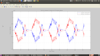
A simulation was run yesterday, with a modified profile of no. of BMRs (Unsigned Flux=2X10^21 Mx) errupting V/s time as below:

Total BMRs per cycle: 7630

The total flux between 2 latitudes was calculated by integrating the product of longitudinally averaged magnetic field and the area of a grid element at that latitude.

                              Flux=Sum[Bavg(lat)*area(lat)]

Flux between any 2 latitudes was thus calculated at regular intervals, and the difference between flux at 2 different times would give us the change in flux, meaning the flux transported. This difference can be interpreted as flux flowing in the concerned region. It can be both positive and negative.

                                                     BUTTERFLY DIAGRAM

                                                     Peak Polar Field: +/- 11 Gauss

The initial polar field in the northern hemisphere was negative, and that in the southern hemisphere was positive.

1. 0-5 :

So, the flux transported to the equator from above 5 degrees latitude would be negative in the northern hemisphere, and positive in the southern. This flux gets cancelled across the equator.

Remember that the calculation of flux transport here, shows the net flux flowing into the concerned region. So, this plot suggests that there is a flow of negative flux(leading polarity) into the northern region, and flow of positive flux(leading polarity) into the southern region. Both flow towards the equator, where these fluxes cancel each other.

The net flux in the region of 5 degrees from the equator can reach the order of 1-2 sunspots.

2. 10-20 :

The flux transport from 10-20 degree latitudes is negative in the northern hemisphere initially, and then becomes positive after half cycle. This is because the BMRs errupt at higher latitudes initially, hence the leading polarity crosses this region on its way to the equator. But, later on, BMRs start appearing at lower latitudes, which results in a net transfer of trailing polarity flux to the poles.

The net flux in this region can reach the order of  1.5X10^22 Mx.

3. 20-30 :

The trailing polarity flux from lower latitudes enters this region, signified by positive peaks in the northern hemisphere (1st cycle) and negative peaks in the southern hemisphere. 

 

The net flux in this region can reach the order of  4X10^21 Mx.

4. 30-40 :

In this region, there is just about no erruption of BMRs. So, this is like a come and go region for flux. The plot here is plotted with the unsigned difference in net flux for simplicity. Positive peaks indicate the trailing polarity flux entering the region, and negative peaks indicate, that a net flux from leading polarities has entered the region. Overall, there is a negligible storage of trailing polarity flux in this region. 

The net flux in this region can reach the order of 6X10^21 Mx. 

5. 40-50 :

There is a lot of addition and subtraction of flux in this region during a solar cycle. A positive peak in the flux transport (1st cycle) indicates the trailing polarity reaching the region, and negative peak indicates that the leading polarity flux has entered the region. Overall, there is a small net accumulation of flux from the trailing polarity in this region. 

The net flux in this region can reach the order of  8X10^21 Mx.

6. 50-60 :

This region comprises partly of the polar field. The plot shows, that there is always a positive net flux reaching this region in the first cycle, which cancels the previous field, and builds up a new one. Then, for the next cycle, there a negative flux reaching this region at all times. So, the net flux in this region does not show more than one peak. If it is increasing, it will increase till the highest value, and if it is decreasing, it will decrease till the lowest value. 

The net flux in this region can reach the order of  2.5X10^22 Mx.

2 Different Butterfly Diagrams

All the Butterfly diagrams till now were plotted with latitude on the y axis, and time on the x axis. But normally data analysts plot the butterfly diagrams with sine of the latitude on the y axis.

This post is to show what difference is created by changing the axis.

                                                           Latitude V/s time butterfly plot

                                                        Sin(Latitude) V/s time butterfly plot

We can see that in the latter plot, the area from 0 to 60 degree latitude has been magnified, and the area from 60 to 90 degrees latitudes has been compressed near the poles.

Summary of the effect of variation of sunspot paramters

The difference in the peak polar field in consecutive solar cycles varies with different parameters of BMRs as:

1. TILT ANGLE:

Standard tilt angle: 19 degrees (van Ballegooijen et al.)

2. SEPARATION:

Standard separation: Unknown

3. NO. OF SUNSPOTS PER CYLCLE:

Standard no. of sunspots per cycle: Unknown

Observations show the difference in the peak polar field to be around 20 Gauss. Now, several combinations of variations in these parameters can lead us to that difference.

Effect of varying separation in BMRs on the strength of Solar Cycle

The separation between the spots in a BMR has a significant effect on the strength of the Solar cycle.
R is the radius of individual sunspots, and 2 sunspots in a BMR are identical, except that they have magnetic field of opposite polarity. All the distances are between centers of sunspots.
1 unit distance=1000km
snomax=200
tilt=lat/2 with sd=19 degrees
Bmax as per Jiang et al.
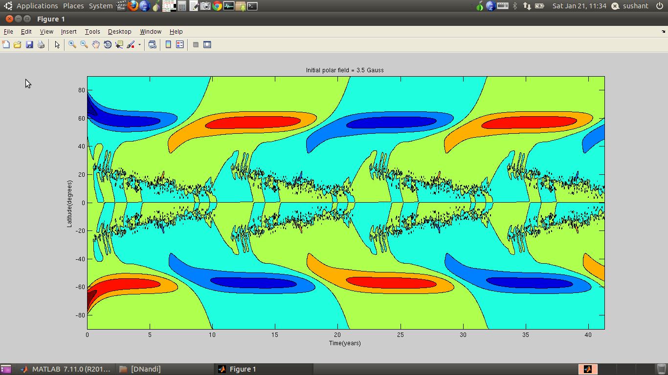
Initial polar field= 3.5G, since this value gives stable(equal) oscillations for no change in parameters.

1. Separation= 2R-10

The magnetic field oscillates between +0.84 G and -2.55 G.
Difference= 3.39 G


2. Separation= 2R-5

The magnetic field oscillates between +1.6 G and -2.54 G.
Difference= 4.14 G

3. Separation=2R

The magnetic field oscillates between +2.65 G and -2.55 G.
Difference= 5.20 G

4. Separation= 2R+10

The magnetic field oscillates between +4.011 G and -2.50 G.
Difference= 6.51 G

5. Separation= 2R+20

The magnetic field oscillates between +5.56 G and -2.47 G.
Difference= 8.03 G

6. Separation= 2R+30

The magnetic field oscillates between +6.85 G and -2.45 G.
Difference= 9.30 G


Internal flux cancellation depends on the separation between the 2 spots in a BMR. The greater the separation, less is the cancellation, and more flux is transported towards the poles. Clearly affecting the strength of the cycle.

For every value of separation, there will be a different value of initial polar field, for which we will obtain an oscillation with same magnitude on either side of zero. But the difference between the peaks will stay the same, as previous simulations suggest.

Modified Separation

All the previous simulations were for  a larger separation between 2 sunspots in a BMR, so that maximum flux is differentially transported.

But now, to study the effect of varying the no. of sunspots per cycle, we need to fix the separation at some value.

For the next post, that will cover the variation of peak magnetic field with respect to variation in no. of errupting BMRs in a cycle, the separation will be fixed such that, the 2 sunspots in a BMR grace each other's boundaries. i.e. separation between their centres is twice their radius. For such a separation, stabilised oscillation is obtained for:

Initial field=3G
The field oscillates between +2.20 and -2.21G
Difference=4.41G

Note: This post should have been before the one below.
The post showing the effect of varying sunspot nos. is below.

Running the code with different number of BMRs per cycle

The code was run with different values of input BMRs per cycle, and the initial field was varied for each run to get a stable oscillation. The results are:

1. No. of BMRs per cycle = 7028,  with a peak of 200 BMRs@5.5 yrs.

Initial field = 3.5G
The field oscillates between +2.65G and -2.55G
Difference=5.20G

2. No. of BMRs per cycle = 10722, with a peak of 300 BMRs@5.5 yrs.

Initial field = 5G
The field oscillates between +3.81G and -3.64G
Difference=7.45G

3. No. of BMRs per cycle = 14412, with a peak of 400 BMRs@5.5 yrs.

Initial field = 7G
The field oscillates between +5.31 and -5.10
Difference= 10.41G

4. No. of BMRs per cycle = 18082, with a peak of 500 BMRs@5.5 yrs.

Initial field = 10G
The field oscillates between +6.58 and -7.25
Difference=15.85G

5. No. of BMRs per cycle = 21768, with a peak of 600 BMRs@5.5yrs.

Initial field = 12G
The field oscillates between +8.66 and -8.66G
Difference=17.32G


6. No. of BMRs per cycle = 25442, with a peak of 700 BMRs@5.5yrs.

Initial field = 13.5G
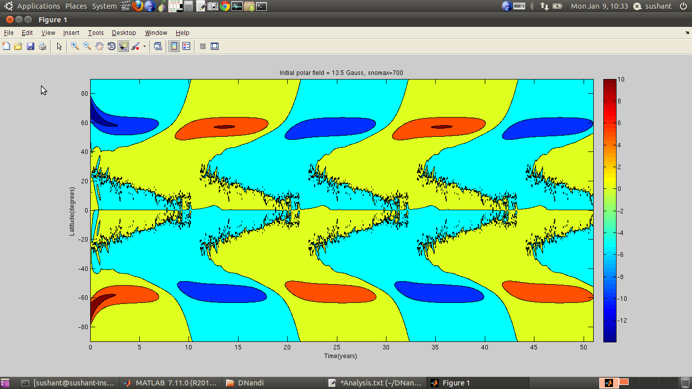
The field oscillates between +10.14 and -9.75G
Difference=19.89G


Ideally, the Sun's peak magnetic field near the poles has a magnitude of about 10G. So, keeping the separation between 2 spots in a BMR to be minimum, so that they just grace each other, we obtain a field of about 10 G in the last case.

Running the code with different initial polar fields

The code was run with different initial polar fields.

1. Initial field of 10 Gauss

OUTPUT:


Peak initial field for the 3rd cycle is -7.55G in the northern hem which occurs at 57.1233 degree lat.@25.3yrs.
The lowest that occurs on the same latitude is -0.86G.@14.2yrs.
Difference=6.7G

So, the cycles go like:

    Year                         Polar field (Gauss)
    14.2                               -0.86
    25.3                               -7.55
    36.4                               -0.86
    47.5                               -7.55


2. Initial field of 9 Gauss

OUTPUT:


Peak initial field for 3rd cycle is -6.7827G in the northern hem which occurs at 57.1233 degree lat.@25.2133yrs.
The lowest that occurs on the same latitude is -0.10699G.@14.1321yrs. and -0.15G.@35.8679yrs.
Difference=6.68G

So, the cycle goes like:

  Year                         Polar field (Gauss)

    14.1                               -0.11

    25.2                               -6.78

    35.9                               -0.15

    47.5                               -6.82

3. Initial field of 8 Gauss

OUTPUT:

Peak initial field for 3rd cycle is -6.06 G in the northern hem which occurs at 57.1233 degree lat.@24.9yrs.

The lowest that occurs on the same latitude is +0.61 G.@14.1yrs. and -0.61G.@35.9yrs.

Difference=6.67G

So, the cycle goes like:

  Year                         Polar field (Gauss)

    14.1                               +0.61

    24.9                               -6.06

    35.9                               +0.61

    46.7                               -6.06

4. Initial field of 7 Gauss:

OUTPUT:

  Year                         Polar field (Gauss)

    14.1                               +1.41

    25.3                               -5.26

    35.9                               +1.38

    47.3                               -5.28

    58.0                              +1.36

    68.8                               -5.31

Difference=6.67G

5. Initial field of 6 Gauss:

OUTPUT:

Year                         Polar field (Gauss)

    14.1                               +2.16

    25.3                               -4.5

    35.9                               +2.16

    47.3                               -4.5

Difference=6.66G


For realistic result, the difference should be around 20 Gauss.

The input parameters that can be varied to achieve this are:
(1) No. of sunspots per cycle (These were modeled vaguely and hence remain doubtful).
(2) Separation between sunspots within a BMR(taken to be a constant=2R)
(3) The longitudes of eruption are totally random. The degree of randomness can be optimized.

Running the code with decreased randomization for calibration

To relatively stabilize the peak polar magnetic field, the input of one sunspot cycle was repeatedly fed into the surface flux transport code with changing polarity of magnetic field. The initial polar field is 4.5 Gauss above 60 degrees latitude.

The butterfly diagram of the simulation is :

The peak polar magnetic field values are:

Cycle          Peak polar magnetic field in Northern Hem        Peak polar magnetic field in Southern Hem
   1                                 +3.30                                                                         -3.15
   2                                  -3.35                                                                        +3.39
   3                                 +3.30                                                                         -3.15
   4                                  -3.35                                                                        +3.39
   5                                 +3.30                                                                         -3.15
   6                                  -3.35                                                                        +3.39
   7                                 +3.30                                                                         -3.15

The next step: Modelling a realistic input based on observations

For realistic solar cycle simulations, corresponding inputs have to be modeled and fed to the Surface flux transport code.

The modelling was done with reference to the study carried out by Jie Jiang et al. (http://arxiv.org/abs/1102.1266v1) and van Ballegooijen et al. 1998.

The input parameters needed are:

(1) Time of BMR eruption

(2) Latitude of eruption

(3) Tilt angle (with respect to the solar equator)

(4) Longitude of eruption

(5) Radius of individual spots in a BMR

(6) Peak magnetic field (Bmax)

(7) Separation between the centers of the individual spots.

One solar cycle of 11 years was divided in 120 phases. And the sunspots were placed at their respective locations after each phase. The following figure shows the latitude of eruption(in degrees) vs phase that was fed into the surface flux transport code:

An initial polar field of +-4.5 Gauss was placed within 23 degrees of the poles, and the surface flux transport code was given a run for 12 sunspot cycles(132 years). This is what was the output:

This is again a butterfly diagram, but you can really see butterfly like structures in it. The polar magnetic field reversal is clearly evident from the diagram.

But, the problem here is, the magnitude of the peak polar field is not constant. It varies from cycle to cycle.   

No. of Cycle     Peak Magnetic field in the northern hemisphere

        1                                             -4.5

        2                                            +3.8

        3                                            -2.8

        4                                            +5.0

        5                                            -3.8

        6                                            +3.4

        7                                            -3.9

        8                                            +2.7

        9                                            -3.9

       10                                           +3.9

       11                                           -4.9

       12                                           +2.3

       13                                           -5.0

Work up till now: Polar magnetic field reversal

An initial polar field of +-10 Gauss was placed within 20 degrees of the poles, and a BMR was placed in each hemisphere, such that the trailing spot has magnetic field of a polarity opposite to the polar magnetic field in that hemisphere. This automatically set the leading spots of the BMR to be opposite in polarity of magnetic flux.

Such BMRs were placed at regular intervals till the polar magnetic field was totally cancelled, and then became opposite.

The following figure is a butterfly diagram of the simulation. There is nothing like a butterfly in it, it is named like that for a different reason.

On the X-axis is the no. of time steps,

on the Y-axis is the latitude of the surface of the Sun,

and the colors indicate the value of magnetic field on a particular latitude at a particular time(averaged over all longitudes).

Work up till now: Building up of poloidal field

In this video, you can see,
When 2 BMRs in different hemispheres are such that, their leading spots have magnetic flux of the opposite sign, then their flux gets cancelled over the equator. While, the flux of the trailing sunspots is carried to the poles by the meridional flow.

But when the tilt of the BMRs is such that the leading spots have magnetic flux of the same sign, there is no cancellation over the equator, and both the poles end up getting the same polarity of magnetic field.

Work up till now

I have written the Surface flux transport code in FORTRAN77.

It seems to be working fine when I load an input with a single Bipolar Magnetic Region(BMR) placed near the equator. The diffusion seems to blow up the sunspots in size, and the meridional flow(11m/s) carries the poloidal component of the flux to the poles.

The above figures are contour plots of the radial magnetic field on the surface of the Sun. The X-axis is the azimuthal angle(phi) and the Y-axis is the polar angle(theta).