Summary of the effect of variation of sunspot paramters

The difference in the peak polar field in consecutive solar cycles varies with different parameters of BMRs as:

1. TILT ANGLE:

Standard tilt angle: 19 degrees (van Ballegooijen et al.)

2. SEPARATION:

Standard separation: Unknown

3. NO. OF SUNSPOTS PER CYLCLE:

Standard no. of sunspots per cycle: Unknown

Observations show the difference in the peak polar field to be around 20 Gauss. Now, several combinations of variations in these parameters can lead us to that difference.

Effect of varying separation in BMRs on the strength of Solar Cycle

The separation between the spots in a BMR has a significant effect on the strength of the Solar cycle.
R is the radius of individual sunspots, and 2 sunspots in a BMR are identical, except that they have magnetic field of opposite polarity. All the distances are between centers of sunspots.
1 unit distance=1000km
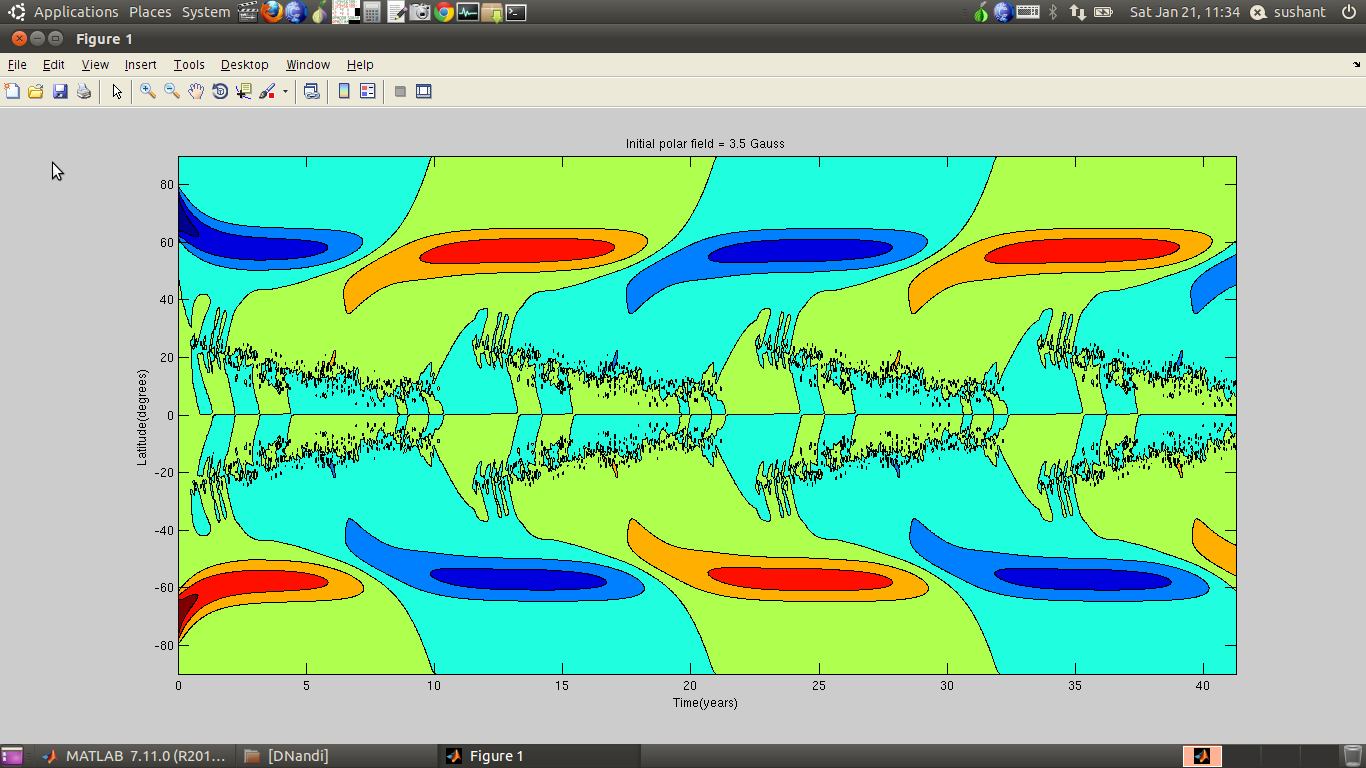
snomax=200
tilt=lat/2 with sd=19 degrees
Bmax as per Jiang et al.
Initial polar field= 3.5G, since this value gives stable(equal) oscillations for no change in parameters.

1. Separation= 2R-10

The magnetic field oscillates between +0.84 G and -2.55 G.
Difference= 3.39 G


2. Separation= 2R-5

The magnetic field oscillates between +1.6 G and -2.54 G.
Difference= 4.14 G

3. Separation=2R

The magnetic field oscillates between +2.65 G and -2.55 G.
Difference= 5.20 G

4. Separation= 2R+10

The magnetic field oscillates between +4.011 G and -2.50 G.
Difference= 6.51 G

5. Separation= 2R+20

The magnetic field oscillates between +5.56 G and -2.47 G.
Difference= 8.03 G

6. Separation= 2R+30

The magnetic field oscillates between +6.85 G and -2.45 G.
Difference= 9.30 G


Internal flux cancellation depends on the separation between the 2 spots in a BMR. The greater the separation, less is the cancellation, and more flux is transported towards the poles. Clearly affecting the strength of the cycle.

For every value of separation, there will be a different value of initial polar field, for which we will obtain an oscillation with same magnitude on either side of zero. But the difference between the peaks will stay the same, as previous simulations suggest.

Modified Separation

All the previous simulations were for  a larger separation between 2 sunspots in a BMR, so that maximum flux is differentially transported.

But now, to study the effect of varying the no. of sunspots per cycle, we need to fix the separation at some value.

For the next post, that will cover the variation of peak magnetic field with respect to variation in no. of errupting BMRs in a cycle, the separation will be fixed such that, the 2 sunspots in a BMR grace each other's boundaries. i.e. separation between their centres is twice their radius. For such a separation, stabilised oscillation is obtained for:

Initial field=3G
The field oscillates between +2.20 and -2.21G
Difference=4.41G

Note: This post should have been before the one below.
The post showing the effect of varying sunspot nos. is below.

Running the code with different number of BMRs per cycle

The code was run with different values of input BMRs per cycle, and the initial field was varied for each run to get a stable oscillation. The results are:

1. No. of BMRs per cycle = 7028,  with a peak of 200 BMRs@5.5 yrs.

Initial field = 3.5G
The field oscillates between +2.65G and -2.55G
Difference=5.20G

2. No. of BMRs per cycle = 10722, with a peak of 300 BMRs@5.5 yrs.

Initial field = 5G
The field oscillates between +3.81G and -3.64G
Difference=7.45G

3. No. of BMRs per cycle = 14412, with a peak of 400 BMRs@5.5 yrs.

Initial field = 7G
The field oscillates between +5.31 and -5.10
Difference= 10.41G

4. No. of BMRs per cycle = 18082, with a peak of 500 BMRs@5.5 yrs.

Initial field = 10G
The field oscillates between +6.58 and -7.25
Difference=15.85G

5. No. of BMRs per cycle = 21768, with a peak of 600 BMRs@5.5yrs.

Initial field = 12G
The field oscillates between +8.66 and -8.66G
Difference=17.32G


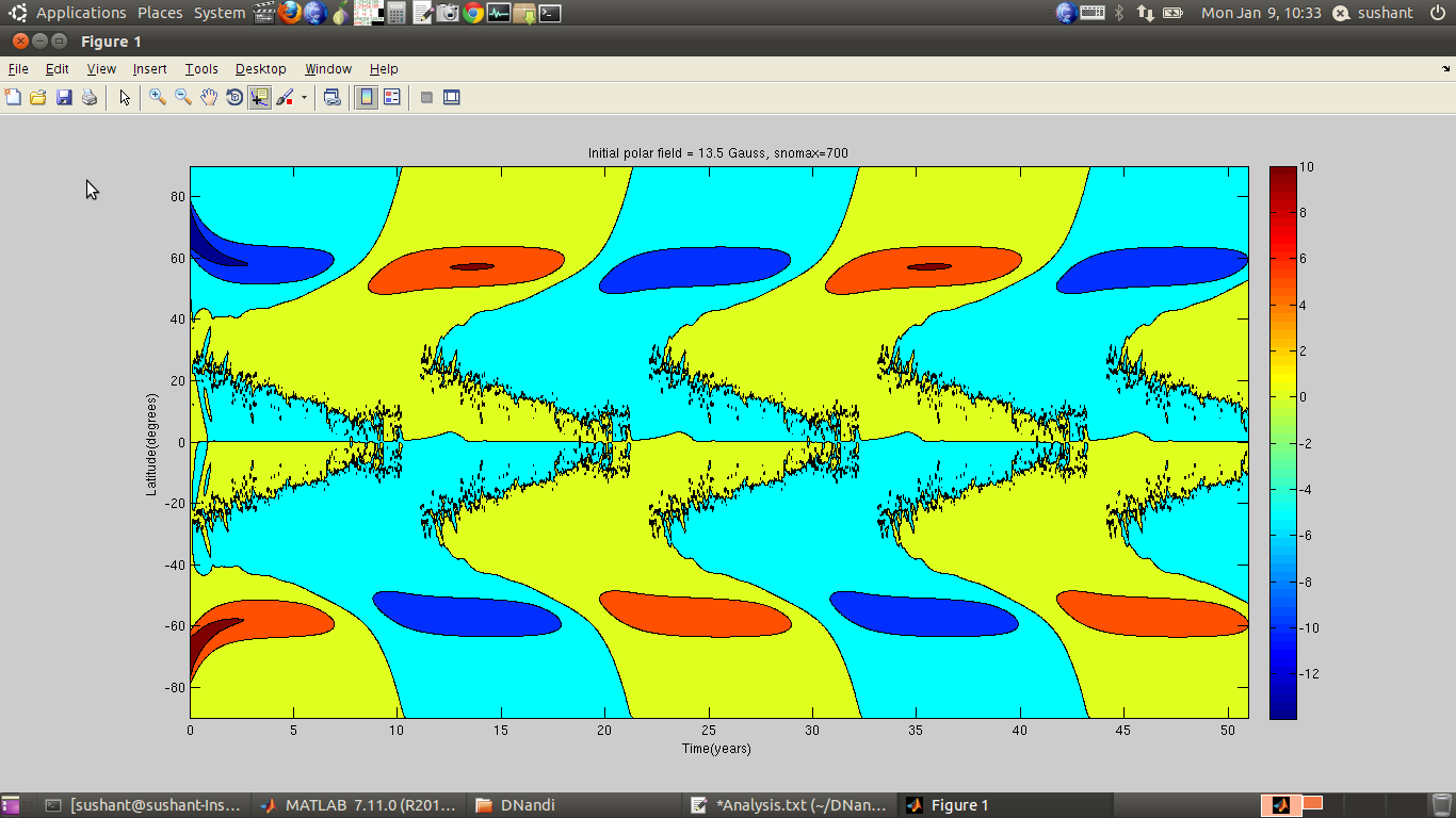
6. No. of BMRs per cycle = 25442, with a peak of 700 BMRs@5.5yrs.

Initial field = 13.5G
The field oscillates between +10.14 and -9.75G
Difference=19.89G


Ideally, the Sun's peak magnetic field near the poles has a magnitude of about 10G. So, keeping the separation between 2 spots in a BMR to be minimum, so that they just grace each other, we obtain a field of about 10 G in the last case.

Running the code with different initial polar fields

The code was run with different initial polar fields.

1. Initial field of 10 Gauss

OUTPUT:


Peak initial field for the 3rd cycle is -7.55G in the northern hem which occurs at 57.1233 degree lat.@25.3yrs.
The lowest that occurs on the same latitude is -0.86G.@14.2yrs.
Difference=6.7G

So, the cycles go like:

    Year                         Polar field (Gauss)
    14.2                               -0.86
    25.3                               -7.55
    36.4                               -0.86
    47.5                               -7.55


2. Initial field of 9 Gauss

OUTPUT:


Peak initial field for 3rd cycle is -6.7827G in the northern hem which occurs at 57.1233 degree lat.@25.2133yrs.
The lowest that occurs on the same latitude is -0.10699G.@14.1321yrs. and -0.15G.@35.8679yrs.
Difference=6.68G

So, the cycle goes like:

  Year                         Polar field (Gauss)

    14.1                               -0.11

    25.2                               -6.78

    35.9                               -0.15

    47.5                               -6.82

3. Initial field of 8 Gauss

OUTPUT:

Peak initial field for 3rd cycle is -6.06 G in the northern hem which occurs at 57.1233 degree lat.@24.9yrs.

The lowest that occurs on the same latitude is +0.61 G.@14.1yrs. and -0.61G.@35.9yrs.

Difference=6.67G

So, the cycle goes like:

  Year                         Polar field (Gauss)

    14.1                               +0.61

    24.9                               -6.06

    35.9                               +0.61

    46.7                               -6.06

4. Initial field of 7 Gauss:

OUTPUT:

  Year                         Polar field (Gauss)

    14.1                               +1.41

    25.3                               -5.26

    35.9                               +1.38

    47.3                               -5.28

    58.0                              +1.36

    68.8                               -5.31

Difference=6.67G

5. Initial field of 6 Gauss:

OUTPUT:

Year                         Polar field (Gauss)

    14.1                               +2.16

    25.3                               -4.5

    35.9                               +2.16

    47.3                               -4.5

Difference=6.66G


For realistic result, the difference should be around 20 Gauss.

The input parameters that can be varied to achieve this are:
(1) No. of sunspots per cycle (These were modeled vaguely and hence remain doubtful).
(2) Separation between sunspots within a BMR(taken to be a constant=2R)
(3) The longitudes of eruption are totally random. The degree of randomness can be optimized.

Running the code with decreased randomization for calibration

To relatively stabilize the peak polar magnetic field, the input of one sunspot cycle was repeatedly fed into the surface flux transport code with changing polarity of magnetic field. The initial polar field is 4.5 Gauss above 60 degrees latitude.

The butterfly diagram of the simulation is :

The peak polar magnetic field values are:

Cycle          Peak polar magnetic field in Northern Hem        Peak polar magnetic field in Southern Hem
   1                                 +3.30                                                                         -3.15
   2                                  -3.35                                                                        +3.39
   3                                 +3.30                                                                         -3.15
   4                                  -3.35                                                                        +3.39
   5                                 +3.30                                                                         -3.15
   6                                  -3.35                                                                        +3.39
   7                                 +3.30                                                                         -3.15

The next step: Modelling a realistic input based on observations

For realistic solar cycle simulations, corresponding inputs have to be modeled and fed to the Surface flux transport code.

The modelling was done with reference to the study carried out by Jie Jiang et al. (http://arxiv.org/abs/1102.1266v1) and van Ballegooijen et al. 1998.

The input parameters needed are:

(1) Time of BMR eruption

(2) Latitude of eruption

(3) Tilt angle (with respect to the solar equator)

(4) Longitude of eruption

(5) Radius of individual spots in a BMR

(6) Peak magnetic field (Bmax)

(7) Separation between the centers of the individual spots.

One solar cycle of 11 years was divided in 120 phases. And the sunspots were placed at their respective locations after each phase. The following figure shows the latitude of eruption(in degrees) vs phase that was fed into the surface flux transport code:

An initial polar field of +-4.5 Gauss was placed within 23 degrees of the poles, and the surface flux transport code was given a run for 12 sunspot cycles(132 years). This is what was the output:

This is again a butterfly diagram, but you can really see butterfly like structures in it. The polar magnetic field reversal is clearly evident from the diagram.

But, the problem here is, the magnitude of the peak polar field is not constant. It varies from cycle to cycle.   

No. of Cycle     Peak Magnetic field in the northern hemisphere

        1                                             -4.5

        2                                            +3.8

        3                                            -2.8

        4                                            +5.0

        5                                            -3.8

        6                                            +3.4

        7                                            -3.9

        8                                            +2.7

        9                                            -3.9

       10                                           +3.9

       11                                           -4.9

       12                                           +2.3

       13                                           -5.0